
COGS 137 Project - The Makings of a Great Scooby-Doo Show
Introduction
For any current or ex-child, the phrase “Saturday Morning Cartoons” most definitely releases a feeling of excitement when heard. After a long week of slaving through the monotonous trenches of school, nothing beats a Saturday morning in front of the television with a bowl of sugary cereal. For generations, television providers have cashed in on this block of time to allow the creation of animated entertainment control the attention of its youth demographic.
On the topic of animation, the continuous output of new cartoons can be recognized as a way of keeping the audience entertained and stationed to their favorite channel. Nevertheless, some cartoons have transcended the short lived cycle to continue their cultural influence in present day.
Scooby-Doo is a children’s mystery series developed by the Hanna-Barbera animation studios in the late 1960s 1. The show follows a group of kids and their dog, with a speech impediment, as they work together to solve mysteries most commonly orchestrated by old people in monster suits. In its over 50 year run, the series has amassed 16 unique television series and over 100 movies 2.
You would imagine that with a ginormous catalog such as Scooby-Doo, it would be impossible to stay invested with every single movie and episode that is offered. Nevertheless, not all heroes wear capes. In assistance with the online Scooby-Doo based encyclopedia, user @plummye completed the entire library of Scooby-Doo that was availabe. In addition, @plummye blessed the internet with a data set of documented variables commonly found in the franchise 3.
Provided with this dataset, our team examined which variables contribute to the IMDB rating. The variables examined in our case study included the network that produced the show, audience engagement in the form of number of IMDB ratings, the format (television episode or movie), monster type, amount of monsters, which character caught the monster, the terrain of the setting, motive, number of times popular character phrases were said, and who the voice actors were for each character.
Question
Which combination of predictor variables in a linear model best predicts the IMDB score for a given Scooby Doo episode/movie?
Load packages
library(tidytuesdayR)
library(tidyverse)
library(tidymodels)
library(broom)
Import Data
tuesdata <- tt_load(2021, week = 29)
scoobydoo <- tuesdata$scoobydoo
Wrangle Data
After looking at the initial dataframe, a lot of the variables can be seen in types of structures and formats that are not optimal for analysis. For our wrangling we changed our variable types to types we could analyze (some sort of numeric/logical value compared to characters). Since there were also some niche crossover and special episodes/series within the dataset that had a different plot-style than normal Scooby Doo episodes/movies, we decided to remove those as well because they would interfere with the analysis of the normal Scooby Doo episodes/movies. We accomplished this by filtering for series names that only contained “Scooby” or “Warner”, and took out special cases where a series had less than three episodes.
# wrangle data
scoobydoo <- scoobydoo |>
  filter(grepl("Scooby", series_name) | grepl("Warner", series_name)) |>
  filter(series_name != "Scooby Goes Hollywood",
         series_name != "The Scooby_Doo Project")

# Most popular phrases
phrases = c("imdb", "engagement", "number_of_snacks", "split_up", "another_mystery", "set_a_trap", "jeepers", "jinkies", "my_glasses", "just_about_wrapped_up", "zoinks", "groovy", "scooby_doo_where_are_you", "rooby_rooby_roo")
scoobydoo[,phrases] <- apply(scoobydoo[,phrases], 2, function(x) as.numeric(x))

people_catch = c("monster_real", 'caught_fred', 'caught_daphnie', 'caught_velma', 'caught_shaggy', 'caught_scooby', "captured_fred", "captured_daphnie", "captured_velma", "captured_shaggy", "captured_scooby", "unmask_fred", "unmask_daphnie", "unmask_velma", "unmask_shaggy", "unmask_scooby", "snack_fred", "snack_daphnie", "snack_velma", "snack_shaggy", "snack_scooby", "trap_work_first", "non_suspect", "arrested")
scoobydoo[,people_catch] <- apply(scoobydoo[,people_catch], 2, function(x) as.logical(x))

amount_monsters = c("monster_amount")
scoobydoo[,amount_monsters] <- apply(scoobydoo[,amount_monsters], 2, function(x) as.character(x))

voice_actors = c("fred_va", "daphnie_va", "velma_va", "shaggy_va", "scooby_va")
scoobydoo[,voice_actors] <- apply(scoobydoo[,voice_actors], 2, function(x) as.character(x))

# create and add monster_catcher column to scoobydoo df
scoobydoo <-
  scoobydoo |>
  mutate(monster_catcher = case_when(
    caught_daphnie == TRUE & caught_fred == FALSE & caught_scooby ==  FALSE & caught_shaggy ==  FALSE & caught_velma == FALSE & caught_other == FALSE & caught_not == FALSE ~ "Daphnie",
    caught_daphnie == FALSE & caught_fred ==  TRUE & caught_scooby == FALSE & caught_shaggy ==  FALSE & caught_velma == FALSE & caught_other == FALSE & caught_not == FALSE ~ "Fred",
    caught_daphnie == FALSE & caught_fred == FALSE  & caught_scooby ==  TRUE & caught_shaggy == FALSE & caught_velma == FALSE & caught_other == FALSE & caught_not == FALSE ~ "Scooby",
    caught_daphnie == FALSE & caught_fred == FALSE & caught_scooby == FALSE & caught_shaggy == TRUE & caught_velma == FALSE & caught_other == FALSE & caught_not == FALSE ~ "Shaggy",
    caught_daphnie == FALSE & caught_fred == FALSE & caught_scooby == FALSE & caught_shaggy == FALSE & caught_velma ==  TRUE & caught_other ==  FALSE & caught_not == FALSE ~ "Velma",
    caught_daphnie == FALSE & caught_fred == FALSE  & caught_scooby ==  FALSE & caught_shaggy ==  FALSE & caught_velma == FALSE & caught_other == TRUE & caught_not ==  FALSE ~ "other character",
    caught_daphnie == FALSE & caught_fred == FALSE  & caught_scooby ==  FALSE & caught_shaggy == FALSE  & caught_velma ==  FALSE & caught_other == FALSE  & caught_not == TRUE ~ "monster not caught",
    TRUE ~ "multiple characters"))
Analysis
Exploratory Data Analysis
Network
Now let’s observe how many Scooby Doo shows each network produced to get a sense for how invested each network was in its Scooby Doo shows.
scoobydoo |>
  group_by(network) |>
  count() |>
  ggplot(aes(x = n,
             y = fct_reorder(network, n),
             fill = network)) +
  geom_col() +
  guides(fill = "none") +
  labs(
    title = "Total Number of Scooby Doo Shows Produced",
    subtitle = "ABC a clear winner in number of shows",
    x = "Number of Shows Produced"
  ) +
  theme_bw() +
  theme(plot.title.position = "plot",
        axis.title.y = element_blank())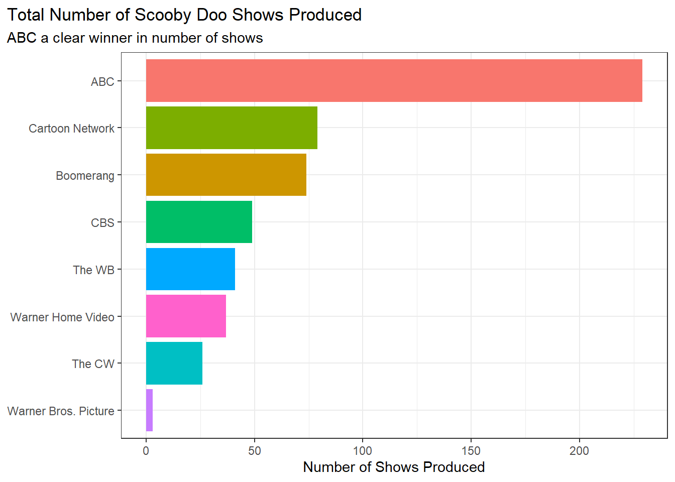
Looking at the number of shows that each network produced, ABC has the most shows, while Warner Bros. Picture has the least.
Engagement Affecting IMDB
Looking at the data, we can see that the number of people that engage with the IMDB website varies per show, and we want to visualize how the number of people that engage could possibly effect the IMDB score. To visualize this, we first filter engagement to be under 10,000 to get rid of the few outliers that would skew the visualization, and use ggplot() and geom_point() to create a scatter plot of the IMDB score compared to engagement numbers.
scoobydoo |>
  filter(engagement < 10000) |>
  ggplot(aes(x = engagement,
         y = imdb)) +
  geom_point() +
  labs(
    title = "IMDB score vs. Engagement Levels",
    subtitle = "IMDB scores skew towards 6-7 as engagement levels increase",
    x = "Number of People Engaged on IMDB Website",
    y = "IMDB Score"
  ) +
  theme_bw() +
  theme(plot.title.position = "plot")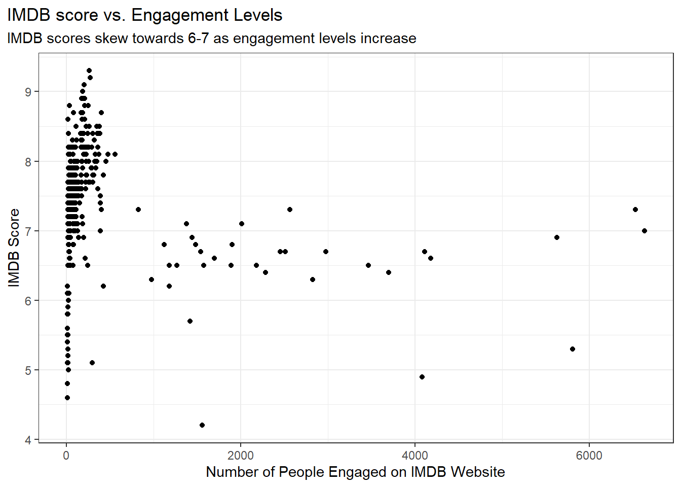
Looking at the data, we see that the shows that received a low amount of engagement had much more variable IMDB scores, which is to be expected since there is a smaller population size and more room for variability. We also saw that when engagement increased, the typical IMDB score was somewhere between 6 and 7, showing that the average score fell within this range when an episode or movie had a high level of engagement on the IMDB website.
Scooby Doo Show Format
Format represents how an instance of the Scooby-Doo show presented to the audience (i.e. televeision episode or movie). Understanding the format of show that the network produced could provide insight into the influence of the show’s format on IMDB score. We checked the count by:
group_by() the dataset by the series format.
count() the number of unique formats
plot a barplot.
scoobydoo |>
  group_by(format) |>
  count() |>
   mutate(format = na_if(format, "NULL")) |>
  drop_na() |>
  ggplot(aes(x = n, y = fct_reorder(format, n), fill = format)) +
  geom_col() +
  guides(fill = "none") +
  labs(title = "Format Types in Scooby-Doo Franchise",
       x = "Number of Times Format is Used", y = "Format Type") +
  theme(plot.title.position = "plot")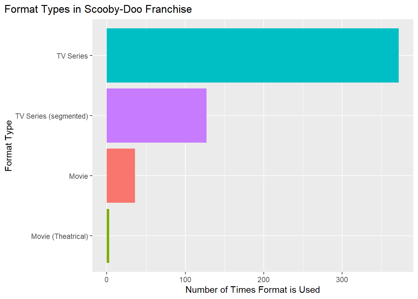
Scooby Doo was intended to be a television series which makes sense why its TV count is over 300 which is far more than the number of movies. Movies were seen as more exclusive and took longer to produce which is why there were not as many.
Monster Type
In every episode of Scooby-Doo, the main characters consisting of Fred, Daphnie, Velma, Shaggy, and Scooby AKA Scooby Doo (collectively self-referred to as “the gang”) have the intention of solving a mystery. While in the process of solving the mystery the gang is usually interrupted by a monster or a villain dressed up as a monster.
Let’s see what monster type the gang encounters the most. We did this by:
group_by() the scoobydoo data set by monster_type
count() the number of times a certain monster type appeared.
mutate() a new column which checked for NULL values and dropped NA values.
filter out any counted monster types that were equal to or less than 11 so we could get the top 10 types.
plot which types were counted the most.
# Determine most common monster type
scoobydoo |>
  group_by(monster_type) |>
  count() |>
  mutate(monster_type = na_if(monster_type, "NULL")) |>
  drop_na() |>
  filter(n >= 11) |> # reduce dataset to top 10 monster_types
  ggplot(aes(x = n, y = fct_reorder(monster_type, n), fill = monster_type)) +
  geom_col() +
  guides(fill = "none") +
  labs(title = "Common Monster Types in Scooby-Doo ",
       x = "Number of Episodes Monster Type Appears In", y = "Monster Type") +
  theme(plot.title.position = "plot")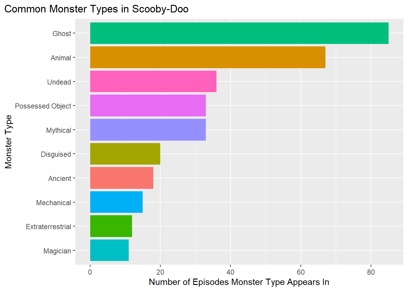
Note that episodes that have multiple monsters are categorized separately. For example, an episode with two ghosts would not count toward the “ghost” total but instead count toward the “ghost,ghost” total.
Based on this plot, it shows that ghosts were the most common monster type. Note that a ghost is a pretty vague type as different people, animals, monsters, etc. can be displayed as having ghost like qualities.
Amount of Monsters
Now let’s look at how many monsters appear in episodes/movies.
scoobydoo |>
  group_by(monster_amount) |>
  count() |>
  ggplot(aes(x = n, y = fct_reorder(monster_amount, n), fill = monster_amount)) +
  geom_col() +
  guides(fill = "none") +
  labs(title = "Number of Monsters Found in an Episode/ Movie",
       x = "Number of Times a Number of Monsters Identified", y = "Number of Monsters") +
  theme(plot.title.position = "plot")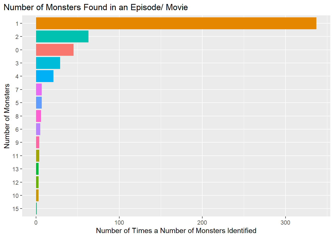
Based on the plot above, we can see that the vast majority of episodes only feature one monster.
Terrain of Setting
The setting of an episode of Scooby Doo was always interesting to find out. With new places around the world also came different types of people that the gang would interact with. We checked this by:
group_by() the dataset by the setting/ terrain variable
count() the number of unique settings
plot a barplot.
scoobydoo |>
  group_by(setting_terrain) |>
  count() |>
  mutate(setting_terrain = na_if(setting_terrain, "NULL")) |>
  drop_na() |>
  ggplot(aes(x = n, y = fct_reorder(setting_terrain, n), fill = setting_terrain)) +
  geom_col() +
  guides(fill = "none") +
  labs(title = "Number of Different Settings Where Show Takes Place",
       x = "Number", y = "Setting/ Terrain") +
  theme(plot.title.position = "plot")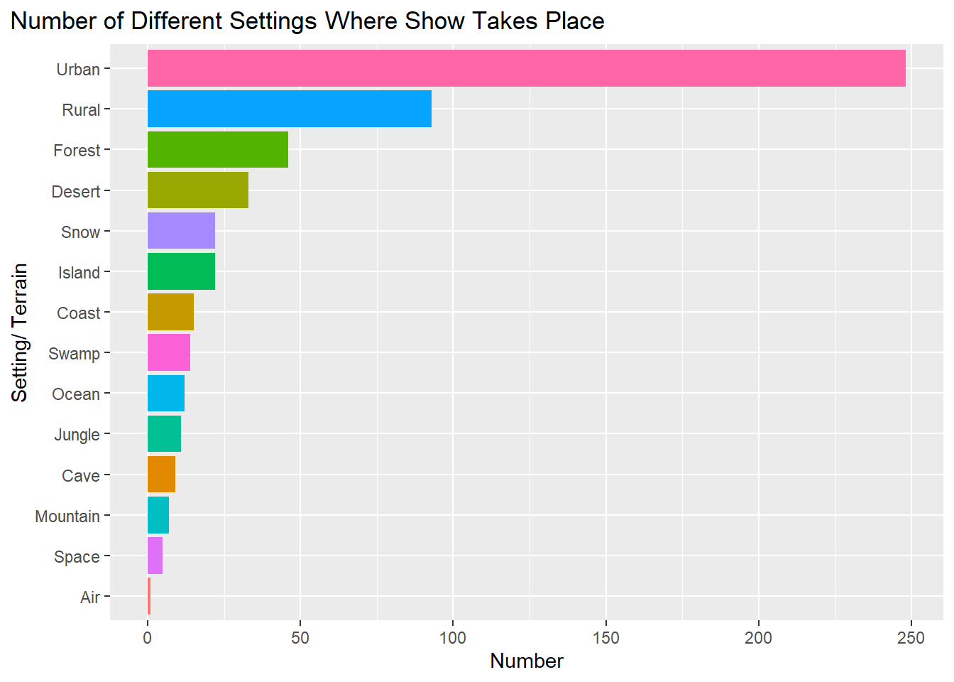
Based on the barplot, urban is the most common setting. All of these settings are vague which could mean that the gang did a lot of their investigations in places with larger groups of people (being in more of a city setting).
Motive
Another variable we checked was the motive behind the crimes committed by the villains in the show. We did this by:
group_by() the dataset by the motive
count() the number of unique motives
plot a barplot.
scoobydoo |>
  group_by(motive) |>
  count() |>
  mutate(motive = na_if(motive, "NULL")) |>
  drop_na() |>
  ggplot(aes(x = n, y = fct_reorder(motive, n), fill = motive)) +
  geom_col() +
  guides(fill = "none") +
  labs(title = "Count of Types of Villian Motives",
       x = "Number", y = "Crime Motive") +
  theme(plot.title.position = "plot")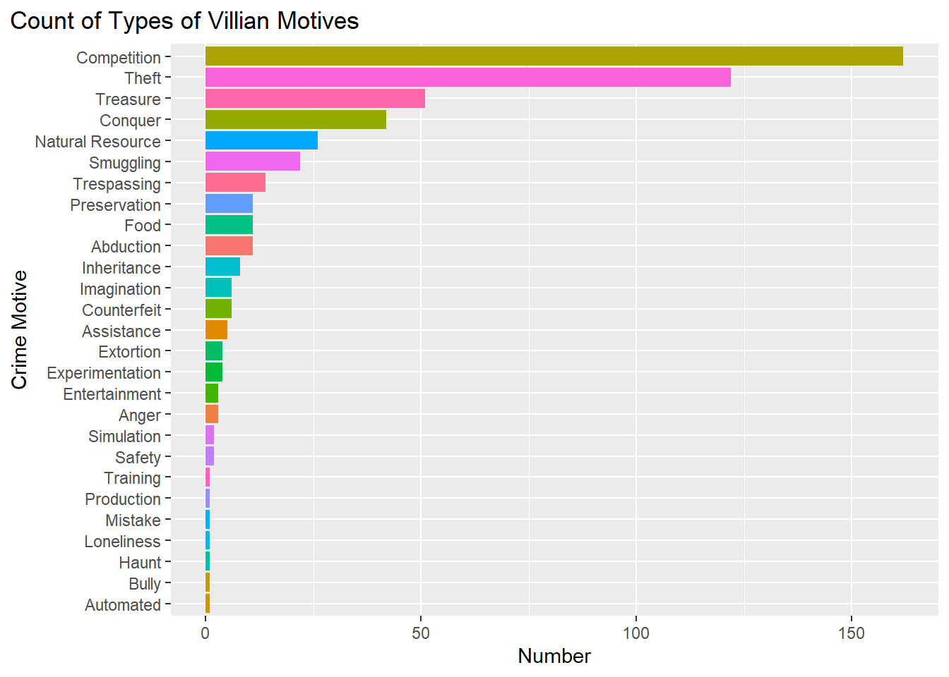
Based on the barplot, the most common reason why a villain would commit a crime was due to competition. These villains would dress up and obstruct society so they could ruin the success or chance of success for another character.
Popular Phrases
It is known that with each character comes their own unique catchphrase that is said in the show. We will track the amounts by:
Use pivot_longer() to take all of the variables of characters saying their phrase and place them as values in the dataset. Select the new pivoted columns that displayed the phrase said the number of times it was said in an episode.
Filter() out the value column to only have phrase that were said more than 0 times.
group_by() the dataset by the name and use summarise() to see how many times a phrase was said.
filter() out all of the unnecessary phrases and included variables that were not necessary for the analysis
Create a plot comparing the number of times a phrase was said.
# most common phrases plot
scoobydoo |>
  pivot_longer(cols = phrases) |>
  select(name, value) |>
  filter(value > 0) |>
  group_by(name) |>
  summarise(count = sum(value, na.rm = TRUE)) |>
  filter(name != "engagement" & name != "imdb" & name != "number_of_snacks" & name != "split_up" & name != "another_mystery" & name != "set_a_trap") |>
  mutate(phrase = case_when(
    name == "zoinks" ~ '"zoinks"',
    name == "jinkies" ~ '"jinkies"',
    name == "rooby_rooby_roo" ~ '"rooby rooby roo"',
    name == "jeepers" ~ '"jeepers"',
    name == "scooby_doo_where_are_you" ~ '"scooby doo where are you"',
    name == "my_glasses" ~ '"my glasses"',
    name == "groovy" ~ '"groovy"',
    name == "just_about_wrapped_up" ~ '"just about wrapped up"')) |>
  ggplot(aes(x = count,
             y = fct_reorder(phrase, count), fill = phrase)) +
  guides(fill = "none") +
  geom_col() +
  labs(
    title = "Frequency of Common Phrases in Scooby Doo",
    x = "Number of Times Phrase is Said",
    y = "Phrase"
  ) +
  theme_bw() +
  theme(plot.title.position = "plot")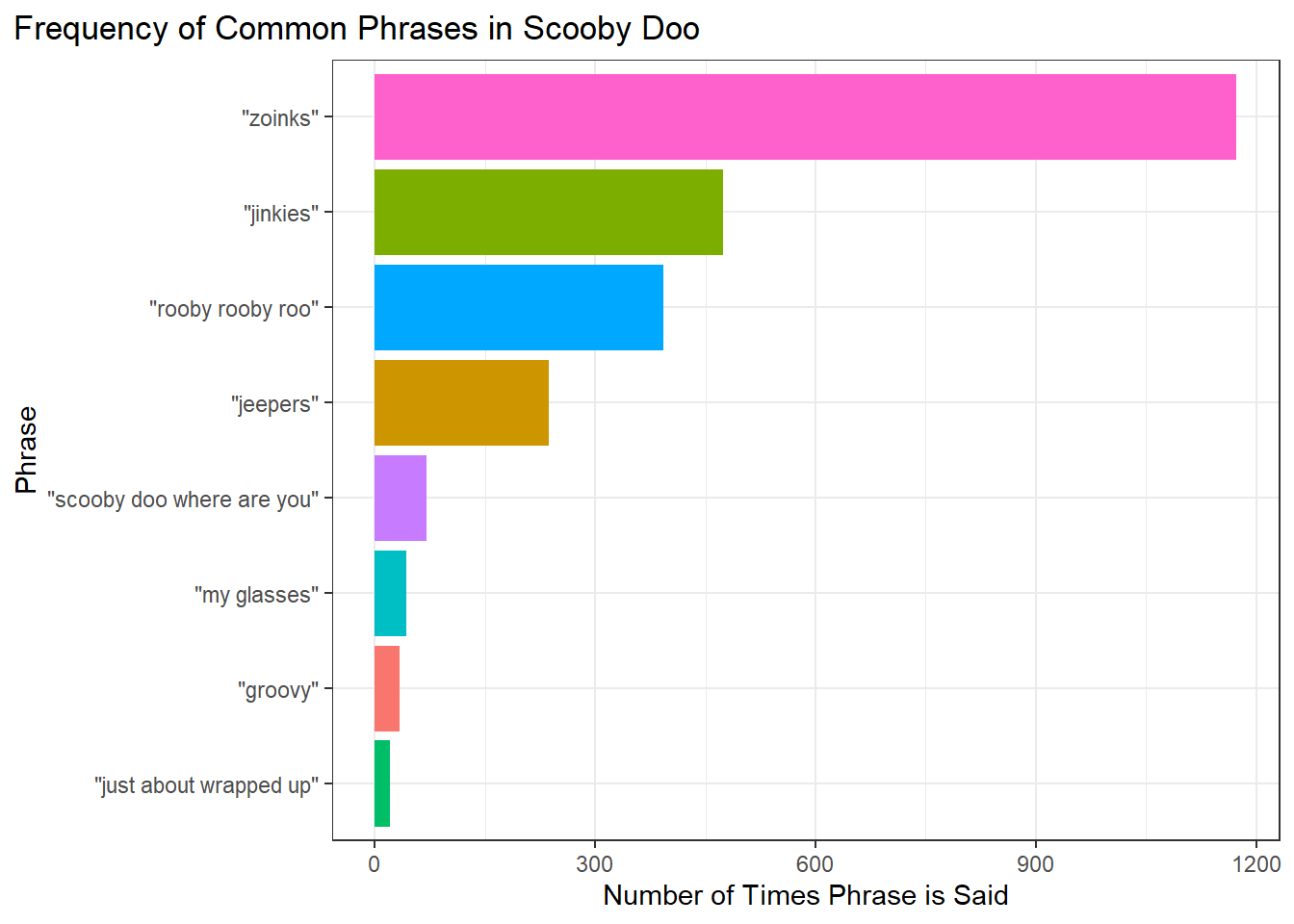
The graph above shows that the phrase “zoinks” is said the most often in the show followed by “jinkies” and “rooby rooby roo”. “Zoinks” is the phrase used by Shaggy in excitement or fear. The same can be said for Velma’s “jinkies”. Finally “rooby rooby roo” is Scooby’s way of exclaiming his own name except that each first letter of every word in his name is replaced with an r.
Who Caught the Monster
We had previously wrangled the data to convert all the variables that tracked the actions of specific characters from character classes to logical classes. These variables were combined and assigned to the name ’people_caught”. Taking this new assigned variable, we then created a new column in the dataset which identified what character had caught the monster in the episode. This worked by identifying what character had a TRUE value in their row for the specific episode and then adding their name in the column. If more than one character had a TRUE for catching the monster, then the column identified that more than one character had caught a monster during that episode To see who had caught the most monsters:
Use pivot_longer() to take all of the variables of characters performing actions and place them as values in the dataset. Select the new pivoted columns that displayed the character and the action they were performing as well as the value of if the action was TRUE or FALSE.
Filter() out the value column to make it that only the TRUE values are present. We don’t care if a character did not catch the monster.
group_by() the dataset by the name and use count() to see how many times TRUE popped up for each character.
select all of the values that started with ‘caught_X’ and add them to a new column where the it just identified their name ‘X’.
Create a plot comparing the number of times each character caught a monster.
# Number of Monsters Each Character Caught Single-handedly
scoobydoo |>
  group_by(monster_catcher) |>
  count() |>
  ggplot(aes(x = n, y = fct_reorder(monster_catcher, n), fill = monster_catcher)) +
  geom_col() +
  guides(fill = "none") +
  labs(title = "Number of Monsters Each Character Caught Single-handedly",
       x = "Number of Monsters Caught", y = "Character") +
  theme(plot.title.position = "plot")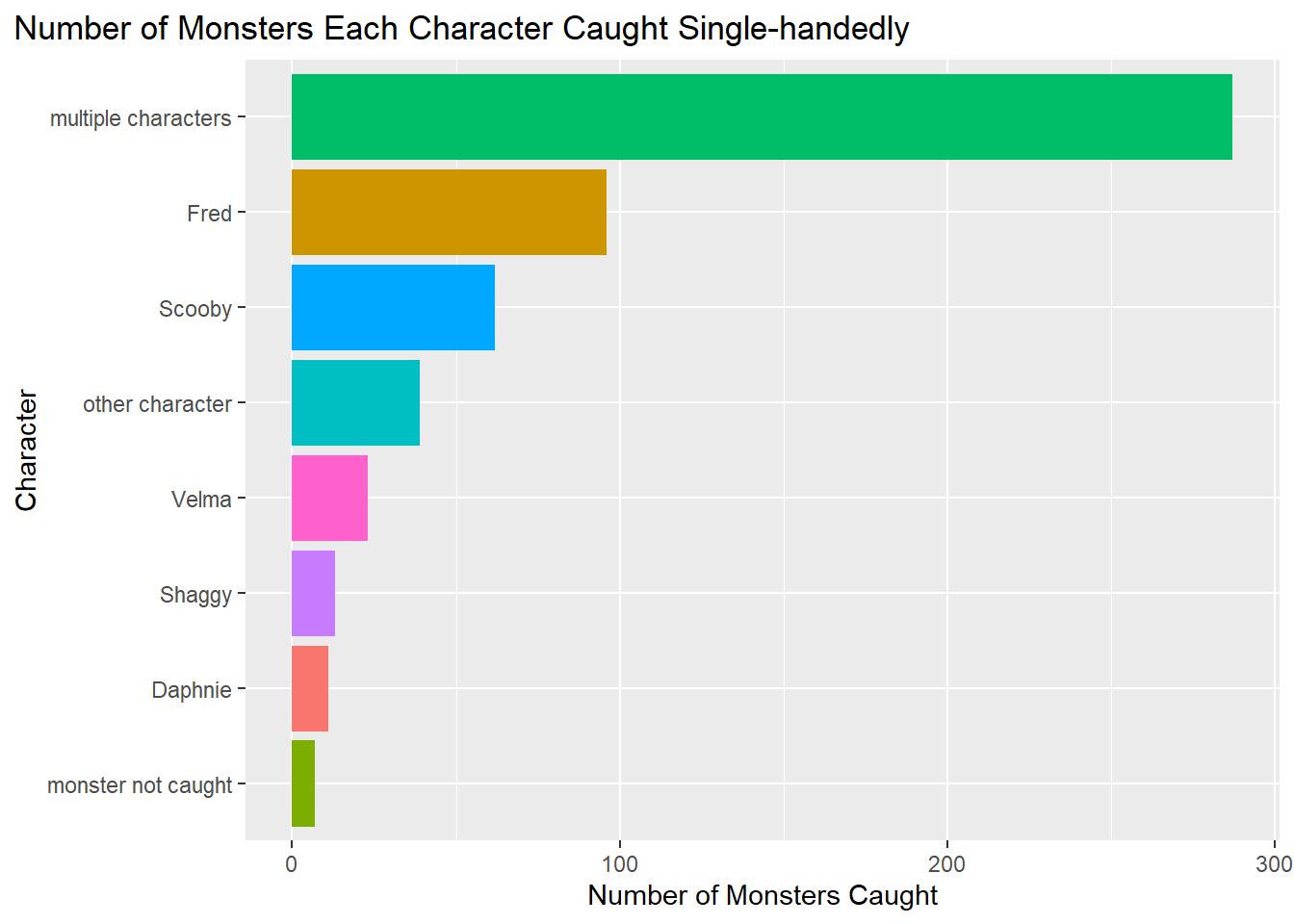
# Number of Monsters Each Character Caught either single-handedly or with others
scoobydoo |>
  pivot_longer(cols= people_catch) |>
  select(name, value) |>
  filter(value == TRUE) |>
  group_by(name) |>
  count() |>
  filter(str_detect(name, "caught")) |>
  mutate(character = case_when(
    name == "caught_daphnie" ~ "Daphnie",
    name == "caught_fred" ~ "Fred",
    name == "caught_shaggy" ~ "Shaggy",
    name == "caught_scooby" ~ "Scooby",
    name == "caught_velma" ~ "Velma")) |>
  ggplot(aes(x = n, y = fct_reorder(character, n), fill = character)) +
  geom_col() +
  guides(fill = "none") +
  labs(title = "Number of Monsters Each Character Caught",
       subtitle = "including single-handedly and with other characters",
       x = "Number of Monsters Caught", y = "Character") +
  theme(plot.title.position = "plot")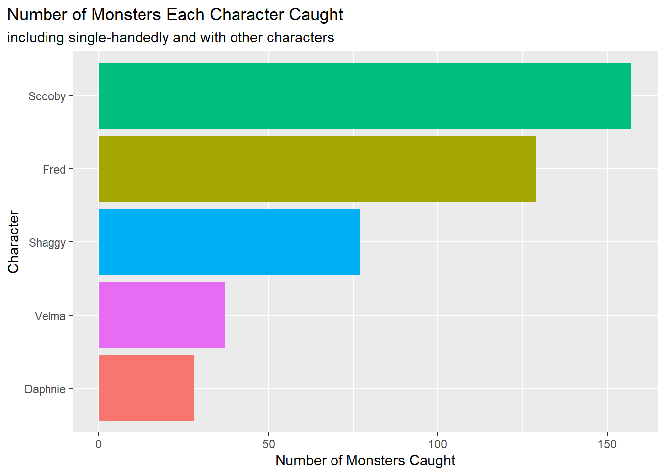
For this portion of the EDA, we chose to create two plots. The first plot takes into consideration the variable of multiple characters working together to catch one monster. Fred single-handedly caught the most monsters. However, when we look at the plot that counts the amount of catches regardless of if a character worked together or alone, Scooby caught the most monsters. Considering this, Scooby was probably often present at times when the group caught a monster. Also it would make sense to have the mascot of the show be a main contributor to catching the monster.
Voice Actors for Each Character
We also wanted to see how many times each voice actor had acted for their character. For each column that identified the voice actor we:
group_by() the dataset by the character’s voice actor
count() the number of unique voice actors
plot a barplot.
#VA Fred
scoobydoo |>
  group_by(fred_va) |>
  count() |>
  mutate(fred_va = na_if(fred_va, "NULL")) |>
  drop_na() |>
  ggplot(aes(x = n, y = fct_reorder(fred_va, n), fill = fred_va)) +
  geom_col() +
  guides(fill = "none") +
  labs(title = "Voice Actor Appearance Count for Fred",
       x = "Number of Appearance", y = "Actor") +
  theme(plot.title.position = "plot")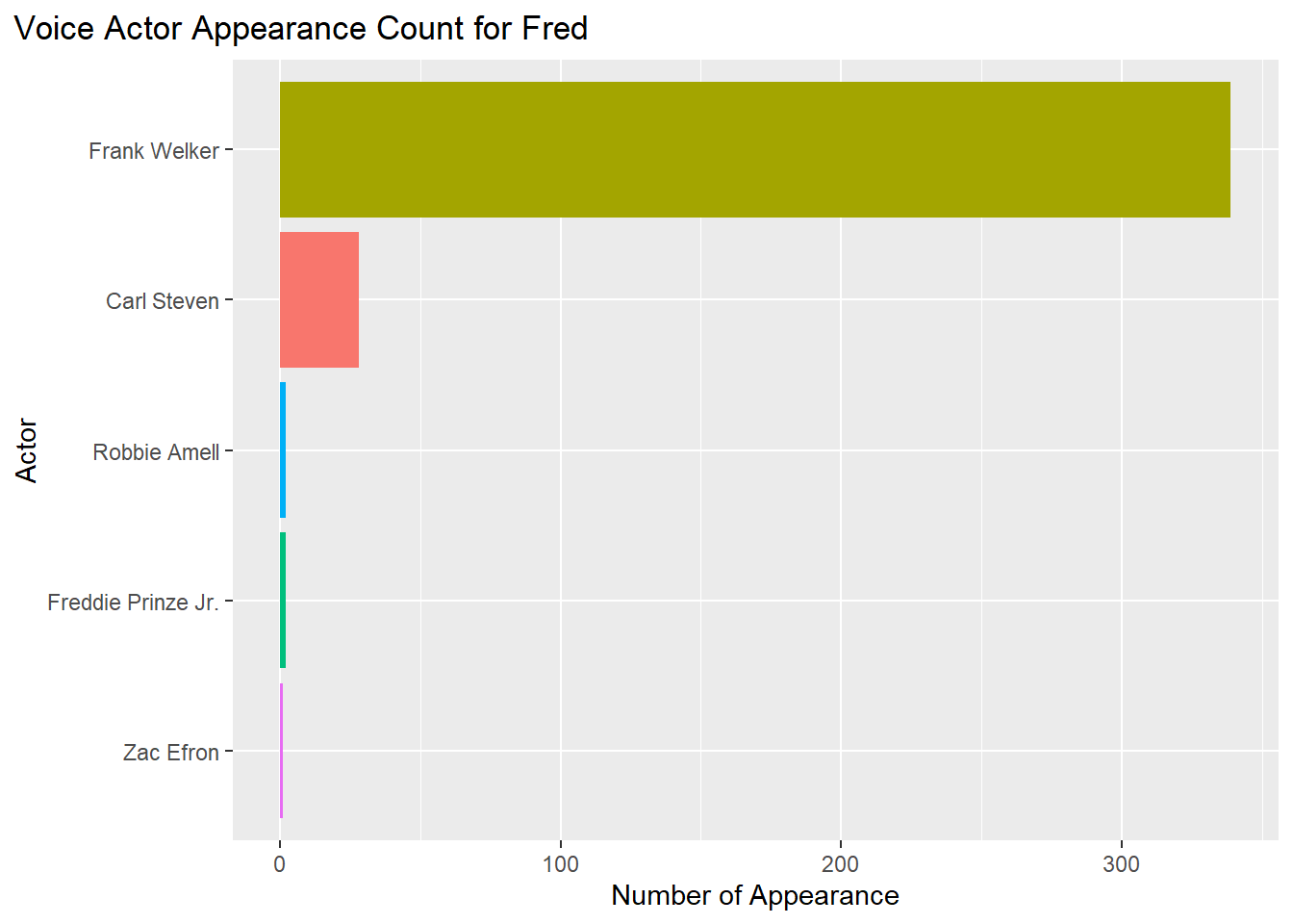
#VA Daphnie
scoobydoo |>
  group_by(daphnie_va) |>
  count() |>
  mutate(daphnie_va = na_if(daphnie_va, "NULL")) |>
  drop_na() |>
  ggplot(aes(x = n, y = fct_reorder(daphnie_va, n), fill = daphnie_va))+
  geom_col() +
  guides(fill = "none") +
  labs(title = "Voice Actor Appearance Count for Daphnie",
       x = "Number of Appearance", y = "Actor") +
  theme(plot.title.position = "plot")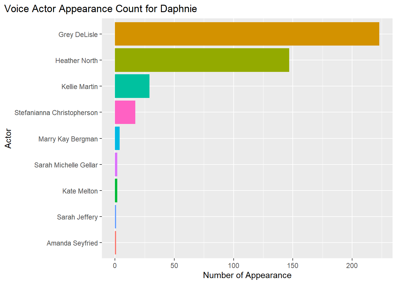
#VA Velma
scoobydoo |>
  group_by(velma_va) |>
  count() |>
  mutate(velma_va = na_if(velma_va, "NULL")) |>
  drop_na() |>
  ggplot(aes(x = n, y = fct_reorder(velma_va, n), fill = velma_va)) +
  geom_col() +
  guides(fill = "none") +
  labs(title = "Voice Actor Appearance Count for Velma",
       x = "Number of Appearance", y = "Actor") +
  theme(plot.title.position = "plot")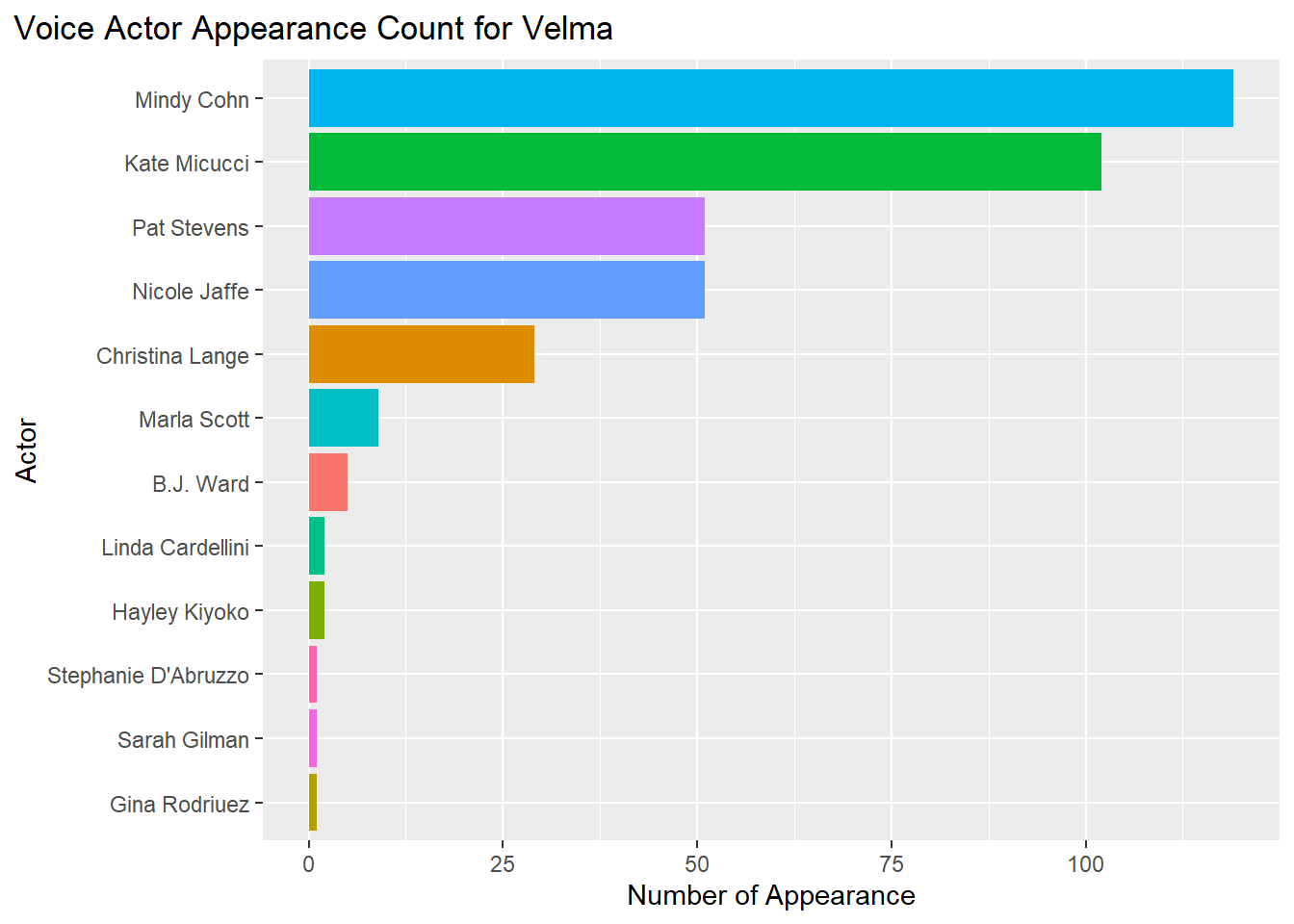
#VA Shaggy
scoobydoo |>
  group_by(shaggy_va) |>
  count() |>
  mutate(shaggy_va = na_if(shaggy_va, "NULL")) |>
  drop_na() |>
  ggplot(aes(x = n, y = fct_reorder(shaggy_va, n), fill = shaggy_va)) +
  geom_col() +
  guides(fill = "none") +
  labs(title = "Voice Actor Appearance Count for Shaggy",
       x = "Number of Appearance", y = "Actor") +
  theme(plot.title.position = "plot")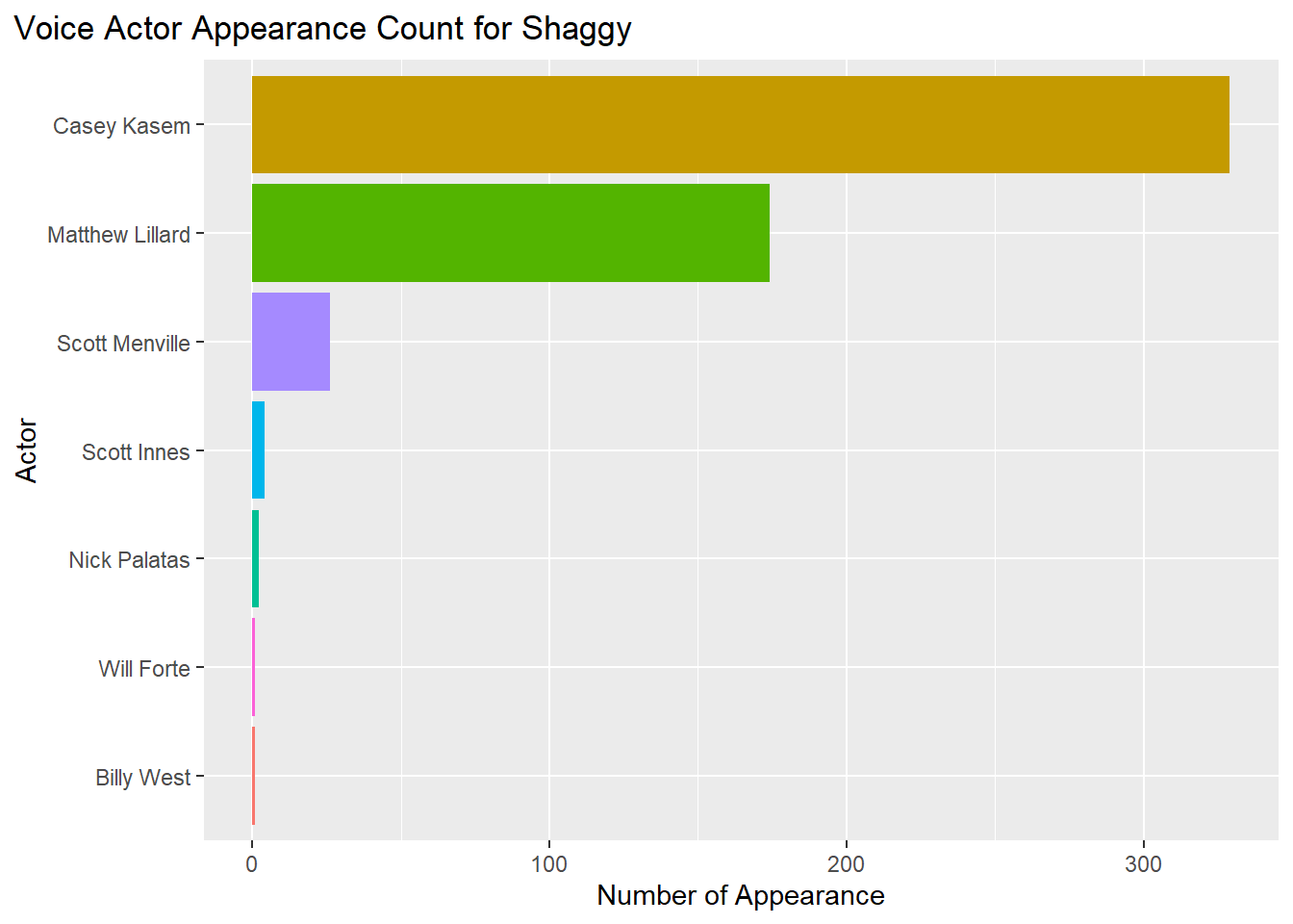
#VA Scooby
scoobydoo |>
group_by(scooby_va) |>
count() |>
mutate(scooby_va = na_if(scooby_va, "NULL")) |>
drop_na() |>
ggplot(aes(x = n, y = fct_reorder(scooby_va, n), fill = scooby_va)) +
geom_col() +
guides(fill = "none") +
labs(title = "Voice Actor Appearance Count for Scooby-Doo",
x = "Number of Appearance", y = "Actor") +
theme(plot.title.position = "plot")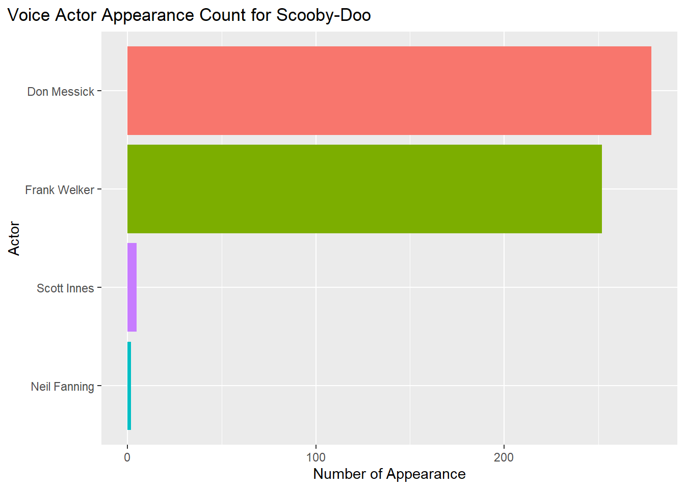 Based on these 5 graphs, here are the voice actors who appeared the most in the franchise.
Fred = Frank Welker (300+ appearances)
Daphnie = Grey DeLisle (200+ appearances)
Velma = Mindy Cohn (100+ appearances)
Shaggy = Casey Kasem (300+ appearances)
Scooby = Don Messick (200+ appearances)
Data Analysis
To test which variables held the greatest weight and helped predict a good IMDB score for a Scooby Doo episode, we utilized a forward selection stepwise regression. The variables we decided to focus on were:
- network
- engagement
- format
- monster_type
- monster_amount
- monster_catcher
- who caught the monster
- setting_terrain
- motive
- zoinks, jinkies, and rooby_rooby_roo
- top 3 iconic phrases, how many times each one was said
- fred_va, daphnie_va, velma_va, shaggy_va, and scooby_va
- who the voice actor was for each character
Starting with the single variable “network” (which had the largest adjusted R squared value out of all other variables to begin with), we added each variable to the linear model and kept whichever single variable increased the adjusted R squared model the most. We continued this pattern until the variables did not increase the adjusted R squared value. The starting adjusted R squared value can be seen below.
rating <-
  linear_reg() |>
  set_engine("lm") |>
  fit(imdb ~ network, data = scoobydoo)
glance(rating)$adj.r.squared
## [1] 0.5803799We continued the pattern of adding a single variable and testing each adjusted R squared value until none of the variables increased the adjusted R squared value on their own. After some iterations, the final linear model’s adjusted R squared that we reached can be seen below.
rating <-
  linear_reg() |>
  set_engine("lm") |>
  fit(imdb ~ network + velma_va + monster_type + motive + engagement + fred_va + zoinks + monster_catcher + monster_amount, data = scoobydoo)
glance(rating)$adj.r.squared
## [1] 0.7367316We can tidy the linear regression dataframe to see which variables help predict a certain increase/descrease in IMDB score as well. The variables that hold weight in predicting an IMDB score are:
- network
- the voice actor for velma
- the type of monster
- motive for crime
- how many people engaged with the IMDB episode website
- the voice actor for fred
- how many times “zoinks” was said
- who caught the monster
- how many monsters were in the episode
tidy(rating)## # A tibble: 198 x 5
## term estimate std.error statistic p.value
## <chr> <dbl> <dbl> <dbl> <dbl>
## 1 (Intercept) 7.12 0.865 8.23 3.86e-15
## 2 networkBoomerang 0.835 0.422 1.98 4.87e- 2
## 3 networkCartoon Network 0.924 0.414 2.23 2.64e- 2
## 4 networkCBS 0.511 0.611 0.836 4.04e- 1
## 5 networkThe CW -1.24 0.576 -2.16 3.14e- 2
## 6 networkThe WB 0.187 0.402 0.465 6.42e- 1
## 7 networkWarner Bros. Picture 6.98 7.29 0.958 3.38e- 1
## 8 networkWarner Home Video -0.247 0.428 -0.576 5.65e- 1
## 9 velma_vaChristina Lange -0.451 0.725 -0.622 5.35e- 1
## 10 velma_vaGina Rodriuez -6.92 6.03 -1.15 2.53e- 1
## # ... with 188 more rowsThere are a lot of rows with different instances and predictors because there are a lot of categorical variables with different options. To sum it up, according to the model, the factors that would indicate a higher IMDB score would be:
- The network was Warner Bros. Pictures
- The voice actor for Velma was Pat Stevens
- The monster types included one ghost, three undead, and three animals
- The motive for crime dealt with inheritance
- The lower the engagement (number of people), the higher the IMDB score
- The voice actor for Fred was Carl Steven
- The more times “zoinks” was said, the higher the IMDB score
- The person who caught the monster was someone other than the five main characters
Results
Of all the models we tested in our forward selection, our analysis showed that the best model was for predicting IMDB rating included the predictor variables: network, Velma’s voice actor, monster type, motive, engagement, Fred’s voice actor, the amount of times “zoinks” was said, and who caught the monster. As the list of predictor variables goes down the list, the weight and effect that each one has on the predicted IMDB score lessens as well.
Looking at the top five most highly rated episodes in the tibble below, we see that our model was wrong on all counts of the expected network, Velma’s voice actor, monster type, motive, engagement level, Fred’s voice actor, number of times “zoinks” was said, and character who caught the monster.
imdb_order <- order(scoobydoo$imdb, decreasing=TRUE)
scoobydoo[imdb_order,] |>
  select(imdb, network, velma_va, monster_type, motive, engagement, fred_va, zoinks, monster_catcher) |>
  slice(1:5)
## # A tibble: 5 x 9
## imdb network velma_va monster_type motive engagement fred_va zoinks
## <dbl> <chr> <chr> <chr> <chr> <dbl> <chr> <dbl>
## 1 9.3 Cartoon Network Mindy Cohn Mythical,An~ Conqu~ 260 Frank ~ 2
## 2 9.2 Cartoon Network Mindy Cohn Ancient Theft 272 Frank ~ 1
## 3 9.1 Cartoon Network Mindy Cohn Mythical Compe~ 202 Frank ~ 0
## 4 9 Cartoon Network Mindy Cohn Mythical Conqu~ 184 Frank ~ 2
## 5 8.9 Cartoon Network Mindy Cohn Mythical Theft 207 Frank ~ 0
## # ... with 1 more variable: monster_catcher <chr>Conclusion
We began this case study by asking which combination of predictor variables in a linear model best predicts the IMDB score for a given Scooby Doo episode/movie. To help answer this question, we explored a variety of variables relevant to the Scooby Doo franchise through various plots in our exploratory data analysis. We then used forward selection to build a linear model with the highest adjusted r squared value. Our final model for predicting IMDB rating takes into account the variables: network, Velma’s voice actor, monster type, crime motive, IMDB engagement, Fred’s voice actor, the number of times “zoinks” was said, which character caught the monster, and the number of monsters in the episode/movie. It was interesting to see that the three top influences on the predicted IMDB score were the network (this had the largest prediction weight), the type of monster, and the voice actor for Velma. Unfortunately, our model did not seem to be very accurate when compared to the top five highest rated episodes in the dataset.
Although we picked many different variables from the original dataset that we thought were most likely to influence the IMDB rating, there were still many variables we did not analyze that likely contributed greatly to the IMDB rating which would explain why our model failed to correctly predict the variable values of the variables included our model for the top 5 most highly rated episodes in the dataset. Also, our case study could be improved by comparing linear models to non-linear models for predicting IMDB score. In a future case study, we would want to look into findings from this case such as how each network handled their episodes of Scooby Doo, how the typical audience perceived the monsters/villains, and how different factors of the voice actor for Velma might have influenced audience perception of the show. We could also look into the factors and situations of the other variables as well, although those had less effect on the predicted IMDB score.